
A complete experiment, from data to decision.
Signal Lab is an interactive engineering demonstrator built by Artificial Modelling. It generates labelled machine telemetry, trains a failure classifier on those generated records, and compares it with a source-trained model on one shared test set. Visitors can change the recipe, inspect alerts, run inference and download the dataset, report and model parameters.
The default experiment generates 6,000 records, including 900 failure-labelled records. Its generated-data model achieves average precision 0.499 versus 0.496 for the source-trained model. The difference is +0.0029. Across five generation seeds, AP varies from 0.489 to 0.520. These results demonstrate retained classification utility in this benchmark; they do not establish a performance advantage.
| Project | Delivered capability |
|---|---|
| Problem | Assess whether generated telemetry retains information useful for rare-failure classification. |
| Data service | Conditional generation, class-balance controls, data checks and reproducible CSV export. |
| Model service | Training, shared-test evaluation, operating-point analysis, inference and parameter export. |
| Delivery | A public browser application, an evaluation snapshot and a documented pipeline. |
Make a feasibility decision before an integration commitment.
Consider a manufacturer or an industrial software team with telemetry from milling equipment and few labelled failures. Before building an alerting workflow, the team needs to understand the labels, establish a baseline, test coverage of uncommon states and decide how many false alarms operators can reasonably review. This is the prospective use case illustrated by Signal Lab.
| Company question | How this project addresses it |
|---|---|
| Can we create useful labelled examples? | Fit conditional distributions and control failure-labelled share; evaluate the resulting model rather than judging records by appearance alone. |
| What will operators have to review? | Show alert counts, correct alerts and missed failures at explicit thresholds. |
| Can our engineers inspect the handover? | Export records, configuration, metrics, coefficients, feature transformations and provenance. |
| What must a pilot establish? | Performance on company-held-out data, useful alert lead time, domain validity and review cost. |
Synthetic examples can support interface testing, scenario exploration and model feasibility work. This experiment tests training on generated data alone. It does not test whether adding generated records to the original training set improves a model; that needs a separate source-plus-generated control.
A useful business evaluation starts with the existing process: inspection rules, operator capacity, current missed events and the action taken after an alert. Agree those measures before choosing a model. The benchmark is a concrete way to discuss that scope, not a forecast of a company’s savings.
One attributed source. Three fixed partitions.
The AI4I 2020 Predictive Maintenance Dataset is distributed by the UCI Machine Learning Repository under CC BY 4.0. It contains 10,000 synthetic records and 339 composite machine-failure labels. The associated introductory paper is by S. Matzka (2020). Source attribution, changes and the original CSV SHA-256 are retained in the data card.
| Partition | Records | Failure labels | Use |
|---|---|---|---|
| Training | 6,000 | 203 | Fit the generator, source classifier and training transforms. |
| Validation | 2,000 | 68 | Choose each model’s initial threshold by maximum F1. |
| Test | 2,000 | 68 | Evaluate both models on the same untouched-by-fitting records. |
Preparation uses Python’s seeded random generator with seed 6841 and a label-stratified 60/20/20 split. Row identities are disjoint across partitions. Identifiers are retained for integrity checks but excluded from prediction. Product ID and the five failure-subtype target columns are also excluded from predictors.
| Input | Representation |
|---|---|
| Product type | L / M / H; M and H indicator features. |
| Air and process temperature | Air temperature and process-minus-air gap, in kelvin. |
| Rotational speed / torque / tool wear | rpm / Nm / minutes. |
| Prediction target | Composite machine failure, encoded 0 or 1. |
Static delivery. Computation in a dedicated browser worker.
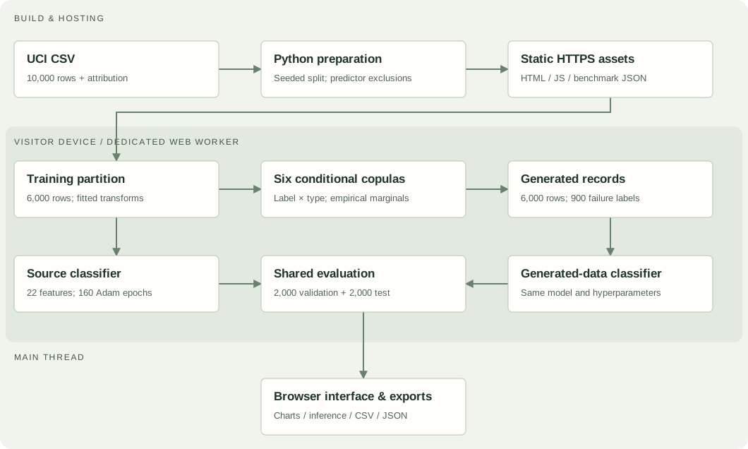
At build time, a Python standard-library script reads the retained CSV, removes leakage-prone predictor fields and emits a fixed benchmark JSON plus a provenance data card. The hosting platform serves HTML, CSS, JavaScript and these public data files over HTTPS.
The interface starts a dedicated Web Worker. The worker loads the benchmark, trains and caches the source model, fits the generator, trains the generated-data model and evaluates both. Progress and result messages return to the interface. A new recipe reuses the cached source model and rebuilds the generated branch.
The main thread renders SVG evaluation charts, a high-DPI three-feature telemetry projection, record previews and score contributions. What-if inference uses the trained coefficients. CSV, report JSON and model JSON are assembled on the device and downloaded as files.
An inspectable statistical pipeline.
The generator fits six Gaussian copulas: one for each failure-label and product-type combination. Within a group, it estimates empirical marginals for air temperature, temperature gap, speed, torque and wear. Tied values use midranks mapped to normal latent scores. The latent correlation matrix keeps a unit diagonal and shrinks off-diagonal correlations by 0.94 before Cholesky sampling.
New correlated latent samples receive Gaussian noise and are normalized by sqrt(1 + noise²). The normal CDF maps them back to empirical quantiles. Product types follow observed proportions within each label. The requested failure count is exact after rounding; fresh IDs and a seeded shuffle complete the dataset. Temperatures and torque are rounded to two decimals; speed and wear to integers.
Both classifiers use the same class-balanced logistic regression with quadratic numeric interactions: five linear features, five squares, ten pairwise products and two type indicators. Each model fits feature standardization on its own training rows. There are 22 transformed features and 23 parameters including the intercept.
| Training choice | Implementation |
|---|---|
| Optimizer | Full-batch Adam, 160 epochs; learning rate 0.035. |
| Adam constants | beta1 = 0.9; beta2 = 0.999; epsilon = 1e-8. |
| Class weighting | n / (2 × class count), calculated separately for each training dataset. |
| Regularization | L2 coefficient 0.005 on non-intercept weights. |
| Feature scaling | Fixed numeric centering/scaling, quadratic expansion, then training-fitted mean/standard deviation. |
| Comparison | Source-only training versus generated-only training; same architecture and hyperparameters. |
Read ranking quality and alert workload together.
Snapshot: 11 October 2026. Default recipe: 6,000 generated rows, 15% failure-labelled share, latent noise 0.15 and generation seed 42. All figures below were reproduced with the same numerical engine used by the live application. Both models are tested on 2,000 source-benchmark rows with 68 failures, a 3.4% positive rate.
| Metric | Source-trained | Generated-data-trained |
|---|---|---|
| Average precision (AP) | 0.496 | 0.499 |
| ROC AUC | 0.951 | 0.939 |
| Initial / last logged weighted training loss | 0.693 / 0.241 | 0.693 / 0.298 |
| Displayed validation-selected threshold | 0.88 | 0.93 |
| Precision at displayed threshold | 45.9% | 68.6% |
| Recall at displayed threshold | 50.0% | 35.3% |
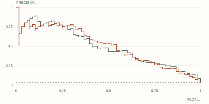
AP summarizes precision across recall increments with tied scores grouped together; the no-skill reference is 0.034. ROC AUC evaluates ranking across both classes. Generated-data training retains similar AP in the default run but has lower ROC AUC. The precision/recall entries use separate model thresholds, so they are not a comparison at a matched alert budget or recall.
| Synthetic threshold | Alerts | Correct alerts | False alarms | Missed failures | Precision / recall |
|---|---|---|---|---|---|
| 0.50 | 281 | 59 | 222 | 9 | 21.0% / 86.8% |
| 0.80 | 95 | 39 | 56 | 29 | 41.1% / 57.4% |
| 0.93 | 35 | 24 | 11 | 44 | 68.6% / 35.3% |
At 0.93, 35 records are flagged: 24 have failure labels and 11 do not; 44 failures are missed. At 0.80, 95 are flagged: 39 correct alerts, 56 false alarms and 29 missed failures. Lowering the threshold in this comparison adds 60 reviews to find 15 additional failure-labelled records. Whether that is worthwhile depends on the operator workflow and consequences of a missed event.
Inspect what changes, and what the checks cover.
| Default generated-data check | Measured result |
|---|---|
| Structurally invalid records | 0 / 6,000 |
| Exact input matches to source training rows | 0 |
| Repeated generated input tuples | 0 |
| Failure-labelled rows | 900 / 6,000 (15.0%) |
| Air temperature KS distance | 0.043 |
| Temperature gap KS distance | 0.038 |
| Rotational speed KS distance | 0.063 |
| Torque KS distance | 0.069 |
| Tool wear KS distance | 0.035 |
Structural checks cover valid type, finite numeric inputs, positive temperature and speed, non-negative torque and wear, and process temperature above air temperature. Exact-match and duplicate checks compare the six input fields, excluding the record ID and label. KS distances compare univariate distributions against source training data. The changed label balance can also change aggregate marginals.
Zero exact copies does not establish anonymity, disclosure safety or a formal privacy guarantee. Univariate KS distances do not establish multivariate fidelity or physical label correctness. A confidential-data project would require an agreed threat model, permissions and appropriate additional tests.
| Noise (fixed seed 42) | AP | ROC AUC |
|---|---|---|
| 0 | 0.509 | 0.939 |
| 0.15 | 0.499 | 0.939 |
| 0.4 | 0.496 | 0.940 |
| 0.8 | 0.500 | 0.940 |
| Generation seed (noise 0.15) | AP | ROC AUC |
|---|---|---|
| 40 | 0.520 | 0.945 |
| 41 | 0.489 | 0.940 |
| 42 | 0.499 | 0.939 |
| 43 | 0.515 | 0.942 |
| 44 | 0.511 | 0.944 |
With row count and label balance fixed, changing noise does not produce a monotonic AP improvement in this small study. Across seeds 40–44, mean AP is 0.507 with sample standard deviation 0.013 and range 0.489–0.520. The source-trained baseline is unchanged. These runs measure generation-seed sensitivity on one test partition; they are not a confidence interval or a statistical superiority test.
Define the decision, then validate it on company data.
| Stage | Company input | Reviewable output / decision |
|---|---|---|
| 1. Scope | Decision, users, event definition, prediction horizon and available history. | Pilot brief with success criteria and data-access responsibilities. |
| 2. Establish | Permitted telemetry, timestamps, machine IDs, event and maintenance logs. | Data audit; time-forward/grouped split; current-rule and source-model baselines. |
| 3. Compare | Rare events, edge cases and domain constraints. | Source-only, generated-only and source-plus-generated controls on representative company holdout. |
| 4. Review | Operator capacity and consequences of errors. | Recall at a fixed alert budget; false alarms per machine/time; lead time; error review. |
| 5. Handover | Integration environment, security and ownership requirements. | Versioned artifacts, inference contract, runbook and shadow-trial plan with human review. |
A pilot should keep a final evaluation window separate from recipe selection. Evaluate by machine, operating regime and failure type where labels support it. Check calibration if probability estimates matter. Review generated records with domain engineers and define monitoring for drift, missing telemetry and changes in equipment.
Artificial Modelling can scope the data preparation, generation, model development, evaluation and handover together. The initial discussion needs a high-level problem description, intended users, available data and success criteria. Data access, timeline, fees, deliverables and ownership are agreed in the project scope.
Reproduce the snapshot
In the project checkout, with Python 3 and Node.js:
python3 build.py
node scripts/check_lab.cjs
node scripts/measure_case_study.cjs
For a browser reproduction, open Signal Lab with its default recipe. Changing settings creates a new run; it does not change this saved case study.
Download exact results JSON ↓Download measurement script ↓Download source data card ↓Source and engine integrity
Source CSV SHA-256
dc6630cd9b1f0f853922fad78a1b6436570d3f1ec863f1dd5c4340ac56bc8a8eNumerical engine SHA-256
982ee7fa67e6e447d99dc555dd86573707f60d531f9da19dbdc3f9c4c6917da6The JSON snapshot also retains preparation, benchmark JSON and measurement-script hashes, exact thresholds, curves, counts and runtime version. The downloadable script is intended for the project checkout; the browser reproduction needs no local setup.
Source and attribution
AI4I 2020 Predictive Maintenance Dataset, UCI. DOI: 10.24432/C5HS5C. Associated introductory paper: S. Matzka (2020). Licence: CC BY 4.0. Changes: numeric encoding, predictor exclusions, seeded partitions and newly generated training-derived samples. Technical implementation and all new measurements: Artificial Modelling, Signal Lab.